Add title to excel chart 2010 mac

In the Select Data Source dialog box, under Legend Entries Series , select the legend entry that you want to change, and click the Edit button, which resides above the list of the legend entries. In the Series Name box, type either the reference to the cell that contains the desired text, or the legend name that you want to use.

Hi I am stumped. I have graphs in the same file on several different tabs. The horizntal axis is dates that I want to be able to select a minimum and maximum at will. For the graph on one tab when I right click on the horizontal axis I can see the "Bounds" field with min and max listed under Axis Options so it is easy to change the min and max date fields.

For the graph on the next tab, I cannot see the "Bounds" listed under Axis Options. Gotta believe I am missing a simple setting somewhere. OK here is the answer an excel guru found for me. Once I cleaned the data problem solved. Hello thanks much. I have an additional question: How can the axis be fixed and not change when being copied and other data is being entered? I have one graph showing the amount of people in street A, axis bound goes from 1 to I copy this graph in order to keep the layout and enter the amount of people in street B, axis bound modifies itself automatically from 1 to 5, but I want it to stay from 1 to How can I do this?

Thanks in advance. Is there any way to change the chart axis title from all upper case to lower case as the upper case comes by default when I create 'Line with marker' Line graph in excel. Can you tell me how to remove non numeric data when i try to do histogram in excel I have row with date and another are with numbers Format the row in Date and Numeric Thank you in advance: In Excel how do you put the percent along the top In Excel, how do you put the percent along the top I have a bar graph showing actual sales, with a line for the target. I am showing data for the entire year, even though we have only 4 months completed - the reason for this is to show the line as to where we are at to target.

Or change the formatting of the remaining months from my data, so that it would look different for those remaining months. I don't think I can break up the series to show shaded bars for the remaining months - so how can I get the chart to pick up the formatting from the source?

I changed the colour of the remaining months and bolded. Im trying to save a chart as a template to a set size, but when I open the chart from templates it reverts back to standard size, how can I fix this? Good Day I am trying to insert an exstra naam in my chart witch I have colour coded next to my chart I have little blocks witch has got n difrent colour with a name next to it how do I insert the name and in the coloum were I put the amounts.

Is there a way to make the reverse value of axis order dynamic? Thanks to all these great blog entries, I have a dynamic chart that displays different data based on a pulldown option counts or amounts. Counts display in the helper table as positive integers, and amounts display as negative decimals, with custom format to display as currency.

Excel 2010: Insert Chart Axis Title

If I choose inverse order when graphing the amounts, switching back to counts now shows the counts descending from the top of the chart. I'd like to only invert the order when the pulldown reads "amounts" or values are negative. Negating the helper table values can be troublesome, since I use the negative amount to format the vertical axis positives display as integers, negatives display as currency.

Bangladesh 10 I have constructed a histogram in excel using the pivot table. I would like to add to the graph of the regular histogram, the cumulative frequency graph.

Was this information helpful?

Should I add to the pivot table a cumulative frequency column? On ablebits. At the very end, you present the histogram for the frequency distribution with the cumulative frequency distribution added to the graph of the histogram but do not show the steps on how to add the cumulative frequency distribution to the graph using the same pivottable. Your reply is appreciated, Thank You. For the legend, the labels default to 'Series 1', ,Series 2' and so on. How can specific names be allocated to replace 'Series 1', 'Series 2' and so on?

In the Select Data Source box, click on the legend entry you want to change, and then click the Edit button. The Edit Series dialog window will show up. The Series name box contains the address of the cell from which Excel pulls the label. You can either type the desired text in that cell, and the corresponding label in the chart will update automatically, or you can delete the existing reference and type the reference to another cell that contains the data you want to use as the label.

E-mail not published. Customizing Excel charts: Add the chart title Customize chart axes Add data labels Add, hide, move or format chart legend Show or hide the gridlines Edit or hide data series in the graph Change the chart type and styles Change the default chart colors Swap vertical and horizontal axes Flip an Excel chart from left to right 3 ways to customize charts in Excel If you've had a chance to read our previous tutorial on how to create a graph in Excel , you already know that you can access the main chart features in three ways: Right-click the chart element you would like to customize, and choose the corresponding item from the context menu.

Use the chart customization buttons that appear in the top right corner of your Excel graph when you click on it. For immediate access to the relevant Format Chart pane options, double click the corresponding element in the chart. To revert back to the original number formatting the way the numbers are formatted in your worksheet , check the Linked to source box.

How to add titles to charts in Excel - in a minute.

October 29, at 1: Bruce says: May 5, at 8: Hi Svetlana I like the way you use arrows to show the sequence of clicks needed to get to a menu item. Thank you Bruce. Arpaporn says: September 15, at 6: Svetlana Cheusheva says: September 15, at Hi Arpaporn, To change the text in the chart legend, do the following: Right-click the legend, and choose Select Data in the context menu.

Thank you very much, Svetlana. I now can change the text in the chart legend.

• flush dns mac snow leopard?
• ERC Tweets.
• ion vcr to pc mac.
• how to make a pdf file smaller to email on mac!

Dennis Baker says: September 23, at 3: Thanks in advance for your help! September 23, at 5: Steph says: October 20, at 6: November 22, at 7: Bikash says: December 8, at 1: Hi there, Is there any way to change the chart axis title from all upper case to lower case as the upper case comes by default when I create 'Line with marker' Line graph in excel. Thanks Bikash. Vesela says: January 31, at 4: David says: February 28, at 8: February 28, at 9: Kim says: May 25, at 5: July 12, at 6: Eva says: September 8, at 6: Does anyone know how to stop the removal of formatting when saving as text in another file?

November 21, at December 21, at Mikey says: January 25, at 4: Thank you all so much for the blog. NIck says: February 9, at 3: Dhiraj says: February 27, at Supriya says: August 27, at August 28, at 9: Hi Supriya, Sure, you can. Here's how: Amy says: September 11, at 9: Hi Can you write a macro or formula to include the data into the legend next to the series name?

Ioane Alexander says: September 20, at Des Williams says: October 5, at 9: October 5, at Hi Des, Here are the steps to change the legend labels: Right-click the legend, and click Select Data… 2. Post a comment Click here to cancel reply. Unfortunately, due to the volume of comments received we cannot guarantee that we will be able to give you a timely response.

When posting a question, please be very clear and concise. We thank you for understanding!

Add-ins for Microsoft Excel - Calculate dates and time See all products. Add-ins Collection for Outlook These 8 tools will boost your inbox productivity and simplify your emailing routine. Plug-ins for Microsoft Outlook - Press the Enter button. So now if I change the text in cell B2 , the chart title will be automatically updated.

A chart has at least 2 axes: When the values don't speak for themselves you should include axis titles to clarify what your chart displays. From Axis Title options choose the desired axis title position: Primary Horizontal or Primary Vertical. In the Axis Title text box that appears in the chart, type the text that you want. If you want to format the axis title, click in the title box, highlight the text that you want to format and go through the same steps as for formatting a chart title.

Choose one of the solutions below that works best for you to remove a chart or axis title from a chart. In Excel you'll find this option if you click on the Chart Title button in the Labels group on the Layout tab. Solution 2 To clear off the title in no time, click on the chart title or an axis title and press the Delete button.

You can also right-click on the chart or axis title and choose 'Delete' from the context menu. Now you know how to add, format, automate and remove such small but important details as chart and axis titles. Don't forget to use this technique if you want to make a complete and accurate presentation of your work using Excel charts. It's easy and it works! If you want to remove chart labels, where do you find the options to do so within the Design tab Chart Tools? I see that I can use the ''add chart element'' from the tab.

The thing is I like to have that option at the top right of my chart as a plus sign. Though, when I click on my chart, the ''plus sign as much as the 2 other usual options do not appear. It is probobly an easy option to check but I can't figure it out. I'm trying to put the chart title below a pie chart. The title format doesn't allow for this option. When I attempt to move the pie chart further up in it's frame to allow for the insertion of a text box, it only separates the pie slices but does not move.

I also can't seem to lock the size of the pie chart so that I can increase the frame size and insert a text box below.

Customizing Excel charts: add chart title, axes, legend, data labels and more

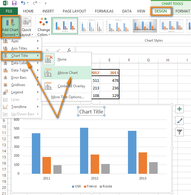
E-mail not published. Add a chart title Format a chart title Make a dynamic chart title Add an axis title Remove a chart or axis title Add a chart title Here's a very simple example how to insert a chart title in Excel Click anywhere in the chart to which you want to add a title. You can see them only if your chart is selected it has a shaded outline. Make a dynamic chart title The time has come for automating the chart title. Click on the chart title. When you type in the equal sign, please, make sure that it is in the Formula bar , not in the title box. Click on the cell that you want to link to the chart title.

The cell should have the text that you'd like to be your chart title as cell B2 in the example below. The cell can also contain a formula. The formula result will become your chart title. You can use the formula directly in the title, but it is not convenient for further editing. Some chart types such as radar charts have axes, but they don't display axis titles. Such chart types as pie and doughnut charts do not have axes at all so they don't display axis titles either. If you switch to another chart type that does not support axis titles, the axis titles will no longer be displayed. November 13, at Madison says: January 31, at 2: Marcus says: September 5, at 5: Marc-Antoine says: December 3, at 9: Fios Huang says: January 10, at 4: Orion says: March 11, at 5: Jennifer says: April 18, at Stan says: June 4, at Wagner Fontes says: December 16, at 7: Post a comment Click here to cancel reply.

Unfortunately, due to the volume of comments received we cannot guarantee that we will be able to give you a timely response. When posting a question, please be very clear and concise. We thank you for understanding!