How to plot a line graph in excel mac

The following steps will create a basic line graph that displays the selected data series and axes. You can then use formatting tools to design the graph to your liking.

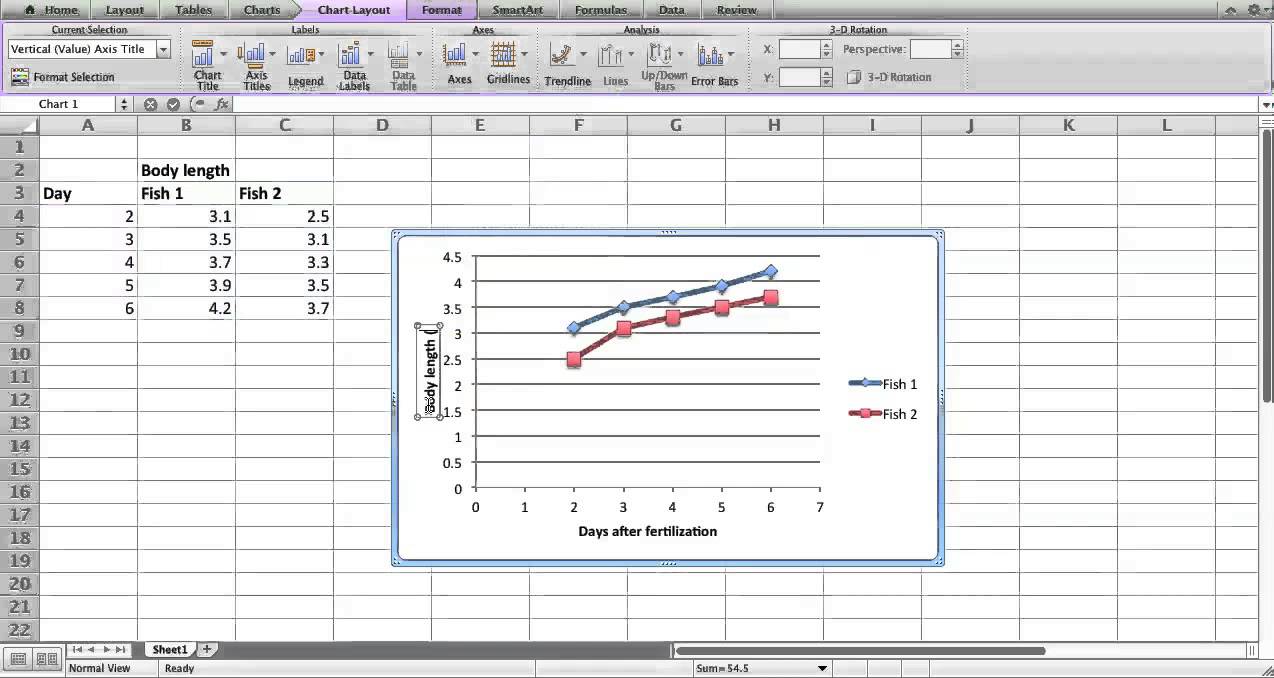
There are many different parts to a chart in Excel — such as the chart title and labels, the plot area that contains the lines representing the selected data, the horizontal and vertical axes, and the horizontal gridlines. All of these parts are considered separate objects by the program, so that you can format them separately. You tell Excel which part of the graph you want to format by clicking on it with the mouse pointer to select it.

If your graph doesn't look like those pictured in this article, it is likely that you did not have the right part of the chart selected when you applied the formatting option. The most common mistake is clicking on the plot area in the center of the graph when the intention is to select the entire chart. The easiest way to select the entire graph is to click in the top left or right corner away from the chart title.

If you make a mistake, it can be quickly corrected using Excel's undo feature. Then, click the correct part of the chart and try again. When you create a chart or graph in Excel or click on an existing graph, two tabs are added to the ribbon as shown in the image above. These Chart Tools tabs — Design and Format — contain formatting and layout options specifically for charts, and you can use them to change the background and text color of the graph. For this graph, formatting the background is a two-step process because a gradient is added to show slight changes in color horizontally across the graph.

Now that the background is black, the default black text is no longer visible. This next section changes the color of all text in the graph to white. The last two steps of the tutorial make use of the formatting task pane , which contains most of the formatting options available for charts.

In Excel , when activated, the pane appears on the right-hand side of the Excel screen as shown in the image above. The heading and options in the pane change depending upon the area of the chart that is selected. Finally, you can also change the formatting of the gridlines that run horizontally across the graph. The basic line graph includes these gridlines to make it easier to read the values for specific points on the data lines.

They do not, however, need to be quite so prominently displayed. One easy way to tone them down is to adjust their transparency using the Formatting Task pane. Share Pin Email. Updated December 18, Click the green Insert tab. Click the "Line Graph" icon. Click a line graph template.

This article was co-authored by our trained team of editors and researchers who validated it for accuracy and comprehensiveness. Microsoft Excel Graphs. Learn more. The wikiHow Tech Team also followed the article's instructions and validated that they work. Learn more Open Microsoft Excel. Double-click the Excel program icon, which resembles a white "X" on a green folder. Excel will open to its home page. If you already have an Excel spreadsheet with data input, instead double-click the spreadsheet and skip the next two steps. Click Blank Workbook. It's on the Excel home page. Doing so will open a new spreadsheet for your data.

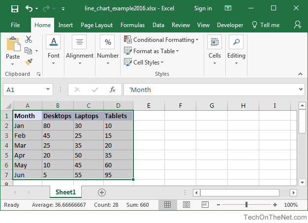
On a Mac, Excel may just open to a blank workbook automatically depending on your settings. If so, skip this step. Enter your data. A line graph requires two axes in order to function. Enter your data into two columns. For ease of use, set your X-axis data time in the left column and your recorded observations in the right column.

For example, tracking your budget over the year would have the date in the left column and an expense in the right. Select your data.

• ip address on mac computer.
• copying outlook files to mac.
• fl studio 10 mac beta download.
• Create and Format a Line Graph in Excel in 5 Steps.
• Creating Line Graphs.
• Was this information helpful?.

Click and drag your mouse from the top-left cell in the data group to the bottom-right cell in the data group. This will highlight all of your data. Make sure you include column headers if you have them. Click the Insert tab. It's on the left side of the green ribbon that's at the top of the Excel window.

How to Make an Excel Chart in Office 2011 for Mac

This will open the Insert toolbar below the green ribbon. It's the box with several lines drawn on it in the Charts group of options. A drop-down menu will appear. Select a graph style.

Graphing a scatter plot or line graph with Mac Excel - Super User

Hover your mouse cursor over a line graph template in the drop-down menu to see what it will look like with your data. You should see a graph window pop up in the middle of your Excel window. Click a graph style. In the Label References field you will see those cells that make the x-axis. The large screen capture below shows this. Next, I added new x-axis data by using mouse pointer to select the data values in my column containing x data. Clicking the header in this instance did not select the entire column - I had to click and drag. After x-axis data had been added I could add the y values in the normal way, by clicking on the header.

Dec 11, The Line Plot is a Category chart.

When you just need a line, there are simple tips to use

The labels on the category x axis are 'categories', not 'values,' and are equally spaced with no regard to the numerical difference from one to the next assuming they are 'numbers'. A Scatter chart has two 'value' axes, and distance from the origin on both is proportional to the values in each series. Scatter charts can show individual data point, with no connection from point to point, or can show the data points connected by line segments or by curves, or can show only the connecting lines, omitting the data points.

Here's a pair of examples, using estimated Y data in the small chart shown in your post. X 'data' has been chosen to demonstrate the differences between a Category chart and an x-y Value chart. Note that the Category labels are in a Header column and the Y data series are in two non-header columns.

1. is mac gargan still venom.
2. Formatting Chart Axes (Mac).
3. Excel line chart (graph);
4. Thank you for your feedback!;
5. Apple Footer.
6. warrior mac daddy 4 goalie gloves;

The selection feeding the chart is rows of columns B and C. Note the spacing of the 'numbers' on the x axis. Note that the blue selection rectangle encloses rows of columns A, B and C, and that the table does not have a Header column. The grey shading in part of column A is applied by Numbers to show these cells are selected—the three unselected cells at the bottom of the table show the default 'no fill' condition of non-header cells.

Note also the horizontal spacing of the data points, and the resulting change in the slope of the lines connecting the data points.



1. free live tv software for mac.
2. How to Plot Two Things on the Same Y Axis in Excel.
3. How to create a line graph in Excel.

The choice of Line Chart vs Scatter Chart should depend not of the perceived aesthetics of the chart as can be seen above, both can have a very similar style , but on which gives a truer picture of the data. For an x-y scatter chart using two series of y values and a shared series of x values, begin by selecting a single x-y pair of columns A and B , then choose the chart type.

With the chart created, and selected, click the Edit Chrt References button below the chart, then go to the table and drag the small white handle right to add the second column of Y values:.

Your Answer

Dec 12, 2: Numbers automatically includes both Ys and automatically sets Share X Values click on bottom left of the numbers window. Plot x-y data in Numbers More Less. Communities Contact Support.