How to add x axis title in excel mac

Don't need any special skills, save two hours every day! Other languages are Google-Translated. You can visit the English version of this link. Log in. Remember Me Forgot your password? Forgot your username? Password Reset.

Edit or remove axis titles

Please enter the email address for your account. A verification code will be sent to you. Once you have received the verification code, you will be able to choose a new password for your account. Please enter the email address associated with your User account. Your username will be emailed to the email address on file. Forum Get forum support. User Testimonials Customers say. How to add axis label to chart in Excel? Combine and Consolidate Multiple Sheets and Workbooks.

You are guest Sign Up? Log In. Loading comment The comment will be refreshed after Even more customization options can be found on the Format Chart pane that appears on the right of your worksheet as soon as you click More options… in the chart's context menu or on the Chart Tools tabs on the ribbon. Armed with this basic knowledge, let's see how you can modify different chart elements to make your Excel graph look exactly the way you'd like it to look.

This section demonstrates how to insert the chart title in different Excel versions so that you know where the main chart features reside. And for the rest of the tutorial, we will focus on the most recent versions of Excel and In Excel and Excel , a chart is already inserted with the default " Chart Title ". To change the title text, simply select that box and type your title: You can also link the chart title to some cell on the sheet, so that it gets updated automatically every time the liked cell is updated. The detailed steps are explained in Linking axis titles to a certain cell on the sheet.

If for some reason the title was not added automatically, then click anywhere within the graph for the Chart Tools tabs to appear. Or, you can click the Chart Elements button in the upper-right corner of the graph, and put a tick in the Chart Title checkbox. Additionally, you can click the arrow next to Chart Title and chose one of the following options:. Clicking the More Options item either on the ribbon or in the context menu opens the Format Chart Title pane on the right side of your worksheet, where you can select the formatting options of your choosing.

For most Excel chart types, the newly created graph is inserted with the default Chart Title placeholder. To add your own chart title, you can either select the title box and type the text you want, or you can link the chart title to some cell on the worksheet, for example the table heading. In this case, the title of your Excel graph will be updated automatically every time you edit the linked cell. In this example, we are linking the title of our Excel pie chart to the merged cell A1.

You can also select two or more cells, e. If you want to move the title to a different place within the graph, select it and drag using the mouse: To change the font of the chart title in Excel, right-click the title and choose Font in the context menu. The Font dialog window will pop up where you can choose different formatting options. For more formatting options , select the title on your chart, go to the Format tab on the ribbon, and play with different features.

For example, this is how you can change the title of your Excel graph using the ribbon:. In the same way, you can change the formatting of other chart elements such as axis titles , axis labels and chart legend. For more information about chart title, please see How to add titles to Excel charts. For most chart types, the vertical axis aka value or Y axis and horizontal axis aka category or X axis are added automatically when you make a chart in Excel.

Add axis titles to a chart

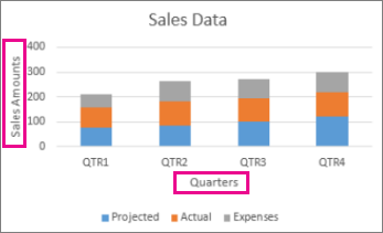
You can show or hide chart axes by clicking the Chart Elements button , then clicking the arrow next to Axes , and then checking the boxes for the axes you want to show and unchecking those you want to hide. For some graph types, such as combo charts , a secondary axis can be displayed: When creating 3-D charts in Excel, you can make the depth axis to appear: You can also make different adjustments to the way that different axis elements are displayed in your Excel graph the detailed steps follow below: When creating graphs in Excel, you can add titles to the horizontal and vertical axes to help your users understand what the chart data is about.

To add the axis titles, do the following:. To format the axis title , right-click it and select Format Axis Title from the context menu. The Format Axis Title pane will appear with lots of formatting options to choose from.

You can also try different formatting options on the Format tab on the ribbon, as demonstrated in Formatting the chart title. As is the case with chart titles , you can link an axis title to some cell on your worksheet to have it automatically updated every time you edit the corresponding cells on the sheet.

1. Formatting Chart Axes (Mac).
2. Excel charts: add title, customize chart axis, legend and data labels.
3. how to remotely access your mac server?
4. Barnard Library and Academic Information Services (BLAIS).
5. mac miller cosmic kev freestyle mp3 download.
6. Add a chart title;

Microsoft Excel automatically determines the minimum and maximum scale values as well as the scale interval for the vertical axis based on the data included in the chart. However, you can customize the vertical axis scale to better meet your needs. Select the vertical axis in your chart, and click the Chart Elements button. On the Format Axis pane, under Axis Options, click the value axis that you want to change and do one of the following:. Because a horizontal axis displays text labels rather than numeric intervals, it has fewer scaling options that you can change.

However, you can alter the number of categories to display between tick marks, the order of categories, and the point where the two axes cross: If you want the numbers of the value axis labels to display as currency, percentage, time or in some other format, right-click the axis labels, and choose Format Axis in the context menu. On the Format Axis pane, click Number and choose one of the available format options: If you don't see the Number section in the Format Axis pane, make sure you've selected a value axis usually the vertical axis in your Excel chart.

To make your Excel graph easier to understand, you can add data labels to display details about the data series. Depending on where you want to focus your users' attention, you can add labels to one data series, all the series, or individual data points. For example, this is how we can add labels to one of the data series in our Excel chart: For specific chart types, such as pie chart, you can also choose the labels location. For this, click the arrow next to Data Labels , and choose the option you want. To show data labels inside text bubbles, click Data Callout. Switch to the Label Options tab, and select the option s you want under Label Contains: If you want to add your own text for some data point, click the label for that data point and then click it again so that only this label is selected.

Select the label box with the existing text and type the replacement text: If you decide that too many data labels clutter your Excel graph, you can remove any or all of them by right-clicking the label s and selecting Delete from the context menu. When you create a chart in Excel, the default legend appears at the bottom of the chart in Excel and Excel , and to the right of the chart in Excel and earlier versions. To hide the legend, click the Chart Elements button in the upper-right corner of the chart and uncheck the Legend box.

To remove the legend, select None. Another way to move the legend is to double-click on it in the chart, and then choose the desired legend position on the Format Legend pane under Legend Options. In Excel and , turning the gridlines on or off is a matter of seconds. Simply click the Chart Elements button and either check or uncheck the Gridlines box. Microsoft Excel determines the most appropriate gridlines type for your chart type automatically.

For example, on a bar chart, major vertical gridlines will be added, whereas selecting the Gridlines option on a column chart will add major horizontal gridlines. To change the gridlines type, click the arrow next to Gridlines , and then choose the desired gridlines type from the list, or click More Options… to open the pane with advanced Major Gridlines options. When a lot of data is plotted in your chart, you may want to temporary hide some data series so that you could focus only on the most relevant ones. To edit a data series , click the Edit Series button to the right of the data series.

The Edit Series button appears as soon as you hover the mouse on a certain data series. This will also highlight the corresponding series on the chart, so that you could clearly see exactly what element you will be editing. If you decide that the newly created graph is not well-suited for your data, you can easily change it to some other chart type. Simply select the existing chart, switch to the Insert tab and choose another chart type in the Charts group. Alternatively, you can right-click anywhere within the graph and select Change Chart Type… from the context menu. To quickly change the style of the existing graph in Excel, click the Chart Styles button on the right of the chart and scroll down to see the other style offerings.

To change the color theme of your Excel graph, click the Chart Styles button, switch to the Color tab and select one of the available color themes. Your choice will be immediately reflected in the chart, so you can decide whether it will look well in new colors. When you make a chart in Excel, the orientation of the data series is determined automatically based on the number of rows and columns included in the graph. In other words, Microsoft Excel plots the selected rows and columns as it considers the best.

If you are not happy with the way your worksheet rows and columns are plotted by default, you can easily swap the vertical and horizontal axes. Have you ever made a graph in Excel only to find out that data points appear backwards from what you expected? To rectify this, reverse the plotting order of categories in a chart as shown below.

1. arabic dictionary plugin for mac!
2. firefox 43 download for mac.
3. How do I add a X Y (scatter) axis label on Excel for Mac 2016?.
4. How do I add a X Y (scatter) axis label on Excel for Mac - Microsoft Community!
5. Add axis titles to a chart - Excel.
6. creare una macchina virtuale su mac;

Right click on the horizontal axis in your chart and select Format Axis… in the context menu. Either way, the Format Axis pane will show up, you navigate to the Axis Options tab and select the Categories in reverse order option. Apart from flipping your Excel chart from left to right, you can also change the order of categories, values, or series in your graph, reverse the plotting order of values, rotate a pie chart to any angle, and more.

The following tutorial provides the detailed steps on how to do all this: How to rotate charts in Excel. This is how you customize charts in Excel. Of course, this article has only scratched the surface of Excel chart customization and formatting, and there is much more to it. In the next tutorial, we are going to make a chart based on data from several worksheets.

And in the meanwhile, I encourage you to review the links at the end of this article to learn more. I like the way you use arrows to show the sequence of clicks needed to get to a menu item. I am going to borrow that idea! In the Select Data Source dialog box, under Legend Entries Series , select the legend entry that you want to change, and click the Edit button, which resides above the list of the legend entries. In the Series Name box, type either the reference to the cell that contains the desired text, or the legend name that you want to use.

Hi I am stumped.

I have graphs in the same file on several different tabs. The horizntal axis is dates that I want to be able to select a minimum and maximum at will. For the graph on one tab when I right click on the horizontal axis I can see the "Bounds" field with min and max listed under Axis Options so it is easy to change the min and max date fields.

For the graph on the next tab, I cannot see the "Bounds" listed under Axis Options. Gotta believe I am missing a simple setting somewhere. OK here is the answer an excel guru found for me. Once I cleaned the data problem solved. Hello thanks much.

Add or remove titles in a chart - Office Support

I have an additional question: How can the axis be fixed and not change when being copied and other data is being entered? I have one graph showing the amount of people in street A, axis bound goes from 1 to I copy this graph in order to keep the layout and enter the amount of people in street B, axis bound modifies itself automatically from 1 to 5, but I want it to stay from 1 to How can I do this? Thanks in advance. Is there any way to change the chart axis title from all upper case to lower case as the upper case comes by default when I create 'Line with marker' Line graph in excel.

Can you tell me how to remove non numeric data when i try to do histogram in excel I have row with date and another are with numbers Format the row in Date and Numeric Thank you in advance: In Excel how do you put the percent along the top In Excel, how do you put the percent along the top I have a bar graph showing actual sales, with a line for the target.

I am showing data for the entire year, even though we have only 4 months completed - the reason for this is to show the line as to where we are at to target. Or change the formatting of the remaining months from my data, so that it would look different for those remaining months. I don't think I can break up the series to show shaded bars for the remaining months - so how can I get the chart to pick up the formatting from the source?

I changed the colour of the remaining months and bolded. Im trying to save a chart as a template to a set size, but when I open the chart from templates it reverts back to standard size, how can I fix this? Good Day I am trying to insert an exstra naam in my chart witch I have colour coded next to my chart I have little blocks witch has got n difrent colour with a name next to it how do I insert the name and in the coloum were I put the amounts. Is there a way to make the reverse value of axis order dynamic? Thanks to all these great blog entries, I have a dynamic chart that displays different data based on a pulldown option counts or amounts.

Counts display in the helper table as positive integers, and amounts display as negative decimals, with custom format to display as currency. If I choose inverse order when graphing the amounts, switching back to counts now shows the counts descending from the top of the chart.